Implementing the Transformer from Scratch for Machine Translation
Tag: Engineering
Published on: 30 Sep 2023
In the ever-evolving landscape of deep learning, the Transformer architecture has emerged as a groundbreaking paradigm shift. Introduced in the seminal paper “Attention is All You Need” by Vaswani et al., the Transformer model has become the backbone of various state-of-the-art natural language processing and autonomous driving applications. In this blog post, we’ll embark on a journey to implement the Transformer from scratch, unraveling its intricacies step by step.
 I heard you are calling my name?
Why Do We Need Transformers
Traditionally, recurrent neural networks (RNNs) are used to solve the natural language processing tasks such as machine translation, where a sequence of text from a source language is being translated into a target language of choice. When producing such sequence of texts, a RNN will keep track of an internal hidden state after producing each token, and uses this state as a hint to produce the next token. This works well for short sentences, but for a longer text information contained in the beginning will be quickly saturated as we move towards the end of the text, making RNNs struggling with capturing long-range dependencies in sequences.
Transformer was introduced to address these limitations, relying on the self-attention mechanism to enable parallelization and capture global dependencies more effectively. With this new model architecture, the model will attend to information extracted from each token simultaneously, which significantly reduces information loss as seen in RNNs.
This can be better understood with the following example, where we aim to translate a text from English to German. For both networks they follow an encoder-decoder architecture where the source text in English is being compressed into some compact representation before being decoded into German. However, for RNNs there is no shortcut in the information flow and in order to produce the German word “siehe” for the German word “seeing” for example, we have to pass 5 network blocks. But for Transformer, each output token now has direct connection to each input token through the self-attention mechanism, essentially reducing the information chain length from 5 to 2 blocks for our example.
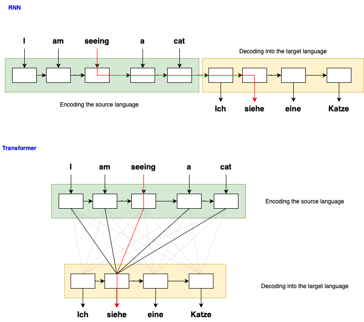 How sequences are produced in RNNs vs Transformers
What is All the Magic in Transformers
The self-attention mechanism (aka. scaled dot-product attention)
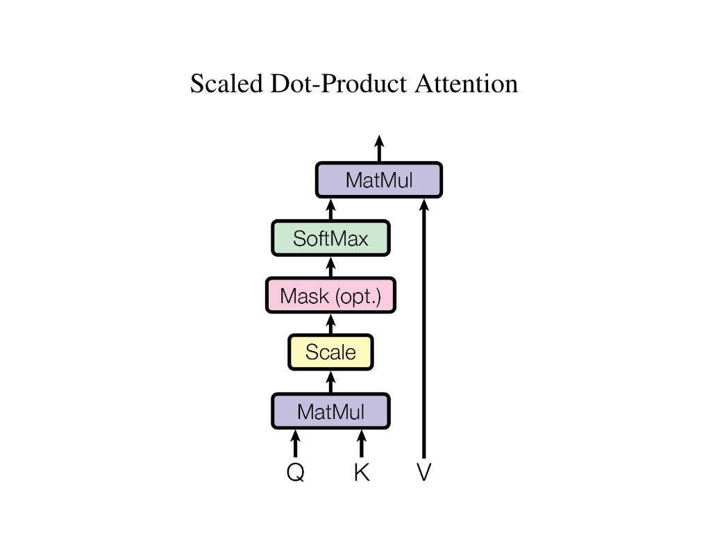 Image Source: Attention is All You Need
In order to understand how the magic happens, we will first need to understand the concept of self-attention, which is the core of the Transformer architecture. Mathematically, the self-attention is defined as:
\[\text{Attention}(Q, K, V) = \text{softmax}(\dfrac{QK^T}{\sqrt{d_k}}) V\]where \(Q\), \(K\), \(V\) are matrices in spaces \(\mathbb{R}^{d_{model} \times d_k}\), \(\mathbb{R}^{d_{model} \times d_k}\) and \(\mathbb{R}^{d_{model} \times d_v}\). Among them, \(K\) and \(V\) represent the keys (what can be provided) and values (what is actually there). In the meantime, \(Q\) represents the query (what is actually needed). All three matrices have a first dimension of \(d_{model}\), which represents the maximum token length the model can represent.
The self-attention mechanism unfolds in two key steps. First, by multiplying \(Q\) with \(K^T\) and then passing the result through a softmax function, we generate an attention matrix of shape \(\mathbb{R}^{d_{model} \times d_{model}}\). Each row in the attention matrix is a probabilistic distribution, indicating how each token \(v_i \in \mathbb{R}^{d_v}\) from \(V\) should be weighted. This step enforces that the model focuses on relevant positions of the encoded sequence. The second step involves multiplying the attention matrix with \(V\), yielding the final output of shape \(\mathbb{R}^{d_{model} \times d_v}\). In this output, each row represents a weighted sum of all rows \(v_i\) from \(V\), effectively consolidating the relevant information based on the attention weights.
The positional encoding
Simply having self-attention isn’t enough to make the Transformer model tick. It’s like missing a crucial puzzle piece—information about where each token sits in the sequence. To fix this, the clever minds behind the Transformer introduced positional encoding. They basically spice up the \(Q, K\) and \(V\) matrices with (co-)sinusoidal signals of different frequencies before these matrices go into the self-attention blender.
To apply positional encoding (PE) to a matrix \(M \in \mathbb{R}^{d_{model} \times d_{feat}}\), they add to each element \(m_{pos,k}\) a PE value of:
\[PE(pos, k=2i) := \sin(pos / 10000^{2i / d_{model}})\] \[PE(pos, k=2i+1) := \cos(pos / 10000^{2i / d_{model}})\]where \(i \in \{0, 1, 2, ...\}\).
Now, why is this a cool move? First off, these (co-)sinusoidal functions keep things in check, hanging out in the range of \([-1, 1]\), so the next layers don’t go wild. Plus, any positional shift \(t\) in the PE can be represented as a linear transformation \(T\) of the original PE: \(PE(pos + t) = T \cdot PE(pos)\), which in theory enables the model to learn position changes as well (derivation). And finally, doing so will not introduce any additional parameters and keeps the dimensions untouched for the input matrix. In the actual implementation, we multiply M by \(\sqrt{d_{feat}}\) before adding the PE to it to make the encoded texts “louder” than the PE. This also explains why we need to throw in a scaling factor of \(1 / \sqrt{d_{feat}}\) later in the attention calculation.
 Image Source: Transformer Architecture: The Positional Encoding
If we attempt to visualize the output of positional encoding, we can also identify its similarity to the binary representation of a number. In binary representation, as we increment a variable, its lowest bit flips first before the higher bits follow suit. When we examine the row vectors generated by positional encoding, we observe a similar pattern: lower dimensions frequently alternate values, whereas higher dimensions show less variation as we increase the position index. Consequently, each position attains a unique combination of values from positional encoding, enabling the model to effectively determine the position of each encoded token.
Positional Masking
When training the transformer, one crucial aspect demands careful attention to ensure the model’s causality during output generation. Causality refers to the property that any output at position \(p\) should solely depend on the outputs from positions \(p' \le p\). During training, when providing the complete sequence as input to the decoder, failing to mask the decoder might lead the model to cheat by peeking into future positions.
To address this, we set all upper triangular elements \(m_{ij}\) where \(j > i\) in the attention matrix \(KQ^T\) to \(-\infty\). This ensures that their probability values become 0 after the softmax layer, essentially excluding these positions from contributing to the final output.
Let’s Code it up
Scaled Dot-product Attention
The scaled dot-product attention function takes three arguments: q, k, and v, which correspond to the query, key, and value tensors, respectively. It employs dot-product to gauge the similarity between the query and key vectors, subsequently combining the values according to the resulting attention matrix.
Optionally, a mask can be provided to exclude specific tokens from participating in the calculation.
def scaled_dp_attention(q: Tensor, k: Tensor, v: Tensor, mask: Optional[Tensor] = None):
	"""
	Arguments:
        q: query tensor of shape (B, seq_len, d_k), with B being the batch size,
            seq_len being the sequence length and d_k being the dimension of the query vector.
        k: key tensor of shape (B, seq_len, d_k)
        v: value tensor of shape (B, seq_len, d_v)
        mask: if given, the tensor elements with a mask value of True will be kept untouched,
            while others will be filled with -inf before the softmax function.

    Output:
        a tuple of (output, attention) where
        output: the output tensor of shape (B, seq_len, d_v)
        attention: the attention tensor of shape (B, seq_len, seq_len)
    """

    d_k = torch.tensor(q.size(-1))
    scores = torch.matmul(q, k.transpose(-2, -1)) / torch.sqrt(d_k)
    if mask is not None:
        scores = scores.masked_fill(~mask, -1e9)
    attention = torch.softmax(scores, dim=-1)
    return torch.matmul(attention, v), attention
Multi-Head Attention
To enhance the attention layer’s capacity for representing information, the authors suggested employing k parallel attention calculations. Each of these calculations yields \(\dfrac{d_{feature}}{k}\) output features, as opposed to relying on a single attention calculation.
class MultiHeadAttention(nn.Module):
    """For an input tensor (B x seq_len x in_features), produce an output tensor with the same dimension.
    """

    def __init__(self, in_features: int, n_heads: int):
	    """
	    Arguments:
		    in_features: number if input features
		    n_heads: number of attention heads
		"""
        super().__init__()

        assert in_features % n_heads == 0, f"the in_features = {in_features} is not divisible by n_heads = {n_heads}"
        self._n_heads = n_heads
        self._in_features = in_features

        # final linear mapping
        self.linear_out = nn.Linear(in_features, in_features)


    def forward(self, q: Tensor, k: Tensor, v: Tensor, mask: Optional[Tensor] = None):
        assert q.shape == k.shape
        assert q.shape[:-1] == v.shape[:-1]
        len_b, len_seq, len_features = q.shape[-3:]
        assert len_features == self._in_features

        q = torch.split(q, self._n_heads, dim=-1)  # list of B x seq x (in_features / h)
        k = torch.split(k, self._n_heads, dim=-1)
        v = torch.split(v, self._n_heads, dim=-1)

        q = torch.concat(q, dim=0)  # concatenate the multi-head dimensions into the batch dimension.
        k = torch.concat(k, dim=0)
        v = torch.concat(v, dim=0)
        if mask is not None:
            mask = torch.concat([mask] * self._n_heads, dim=0)

        x, attn = scaled_dp_attention(q, k, v, mask)  # (h x B) x seq x (in_features / h)
        x = x.view(self._n_heads, len_b, len_seq, len_features // self._n_heads)
        x = x.unsqueeze(-2).swapaxes(0, -2).reshape(len_b, len_seq, len_features).squeeze(0)  # B x seq x in_features

        x = self.linear_out(x)
        return x
Positionwise Feed-forward Layer
The feed-forward layer employs linear mapping to increase the number of features, followed by the application of nonlinearity through the ReLU function. Lastly, another linear mapping is employed to restore the original number of features.
class FeedForward(nn.Module):

    def __init__(self, in_features: int, hidden_features: int, out_features: int):
        super().__init__()
        self._linear_0 = nn.Linear(in_features, hidden_features, bias=True)
        self._linear_1 = nn.Linear(hidden_features, out_features, bias=True)

    def forward(self, x: Tensor):
        x = self._linear_0(x)
        x = torch.relu(x)
        x = self._linear_1(x)

        return x
Positional Encoding
class PositionalEncoding(nn.Module):
    """Module that provides position encoding to an input tensor x of shape (B, MAX_SEQ_LEN, in_features)
    by calculating the sin / cos function value with different time t along the SEQ_LEN dimension
    and different frequency along the in_features dimension"""

    def __init__(self) -> None:
        super().__init__()

    def forward(self, x: Tensor):
        len_feat = x.shape[-1]
        len_pos = x.shape[-2]
        # x is expected to have shape (B, MAX_SEQ_LEN, in_features)
        # where the second and third dimensions correspond to the pos
        # and feature dimension as in the original paper
        pe = torch.zeros((len_pos, len_feat)).to(x)
        feat_idx = torch.arange(0, len_feat)[None, :].float().to(x)  # 1 x len_feat
        pos = torch.arange(0, len_pos)[:, None].float().to(x)        # len_pos x 1
        pe[:, 0::2] = torch.sin(pos / (torch.pow(10000, 2 * feat_idx[:, 0::2] / len_feat)))
        pe[:, 1::2] = torch.cos(pos / (torch.pow(10000, 2 * feat_idx[:, 1::2] / len_feat)))
        self.register_buffer('pe', pe, persistent=True)
        x += pe

        return x
Layer Normalization
In contrast to computer vision tasks, where each input instance (image) has fixed dimensions, natural language processing deals with sentences of varying lengths. Consequently, batch normalization cannot be applied in our machine translation task, as the fluctuating sentence lengths would introduce instabilities in learning the normalization parameters. Instead, the authors employ layer normalization to address this challenge.
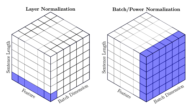 Layer Normalization vs Batch Normalization (Source: Layer Normalizion)
The plot above is sourced from the paper Layer Normalization, demonstrating the distinction between LayerNorm and BatchNorm. For a three-dimensional input \(x \in \mathbb{R}^{d_{batch} \times d_{seqlen} \times d_{feature}}\), batch normalization calculates the running statistics \(\mu_i\) and \(\sigma_i\) over the first and second dimensions independently for each feature \(i\). In contrast, for the layer normalization, the statistics are computed over the feature dimension instead.
class LayerNorm(nn.Module):
    """Normalizes an input tensor of shape (..., in_features) by first computing the mean and standard derivation over the feature dimension.
    Then, apply the learnable parameters alpha and beta individually for each feature dimensions."""

    def __init__(self, in_features) -> None:
        super().__init__()
        self._in_features = in_features
        self._eps = 1e-9
        self._alpha = nn.Parameter(torch.rand(in_features), requires_grad=True)
        self._beta = nn.Parameter(torch.rand(in_features), requires_grad=True)

    def forward(self, x: Tensor) -> Tensor:
        mu = torch.mean(x, dim=-1, keepdim=True)  # calculation over the feature dimension
        sigma = torch.std(x, dim=-1, unbiased=False, keepdim=True)

        x = (x - mu) / (sigma + self._eps)
        x = x * self._alpha + self._beta

        return x
Transformer Encoder
Having assembled the multi-head attention, feed forward, positional encoding, and layer normalization layers, we are now ready to integrate them and construct the Transformer encoder. The architectural diagram below provides a clear blueprint for this process. However, there is one slight adjustment to be made concerning the placement of layer normalization.
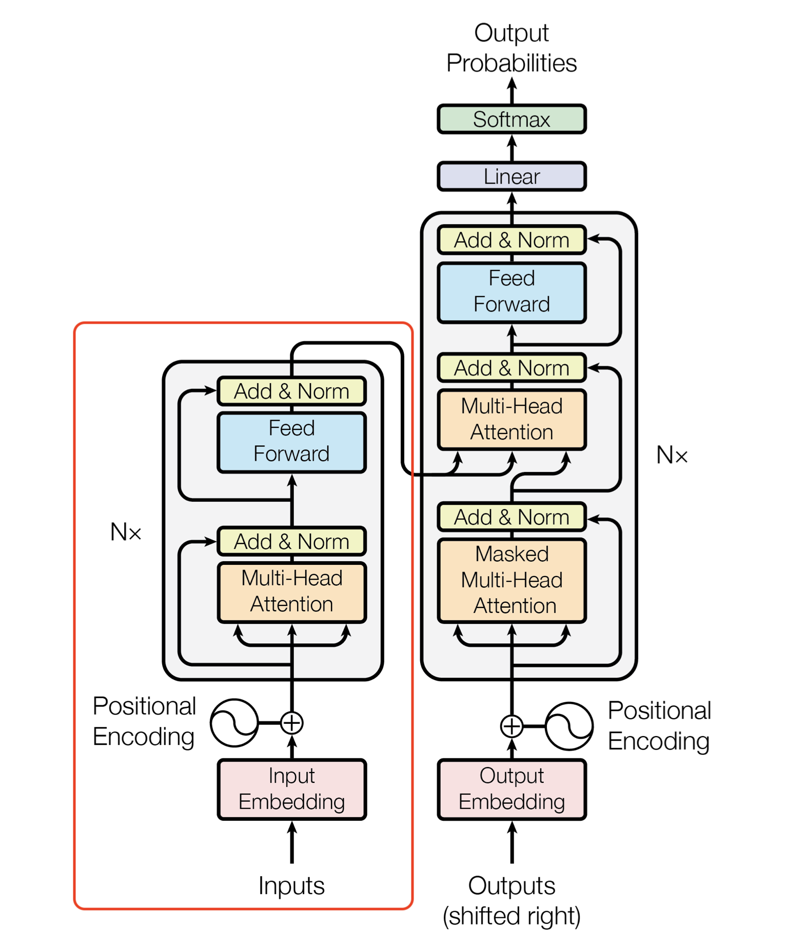 Transformer Encoder Architecture
The diagram, as depicted in the paper, applies LayerNorm after the residual connection. Yet, empirical observations have shown that the network can be trained more efficiently if we move LayerNorm before any sub-layers.
Therefore, we make the following adjustment in implementation:
From: \(x \leftarrow \text{LayerNorm}(x + \text{SubLayer}(x))\) To: \(x \leftarrow x + \text{SubLayer}(\text{LayerNorm}(x))\)
This modification optimizes the training process and enhances the Transformer encoder’s performance.
Furthermore, we employ a dictionary to store all the arguments for the EncoderBlock’s forward pass and return a dictionary as its output. This approach enables us to seamlessly link multiple EncoderBlocks together using the nn.Sequential module.
class EncoderBlock(nn.Module):

    def __init__(self, in_features: int, hidden_features: int, n_attn_heads: int = 8):
        super().__init__()

        self._in_features = in_features
        self._n_attn_heads = n_attn_heads
        self._w_k = nn.Linear(in_features, in_features)
        self._w_v = nn.Linear(in_features, in_features)
        self._w_q = nn.Linear(in_features, in_features)

        self._mh_attn = MultiHeadAttention(in_features, n_attn_heads)
        self._layer_norm_0 = LayerNorm(in_features)

        self._feed_forward = FeedForward(in_features, hidden_features, in_features)
        self._layer_norm_1 = LayerNorm(in_features)

    def forward(self, input: Dict):
        x = input["x"]
        mask = input.get("mask", None)
        x_0 = x
        x = self._layer_norm_0(x)
        k, q, v = self._w_k(x), self._w_q(x), self._w_v(x)
        x = self._mh_attn(k, q, v, mask=mask)
        x += x_0
        del x_0

        x_1 = x
        x = self._layer_norm_1(x)
        x = self._feed_forward(x)
        x += x_1
        del x_1

        return {"x": x, "mask": mask}
Transformer Decoder
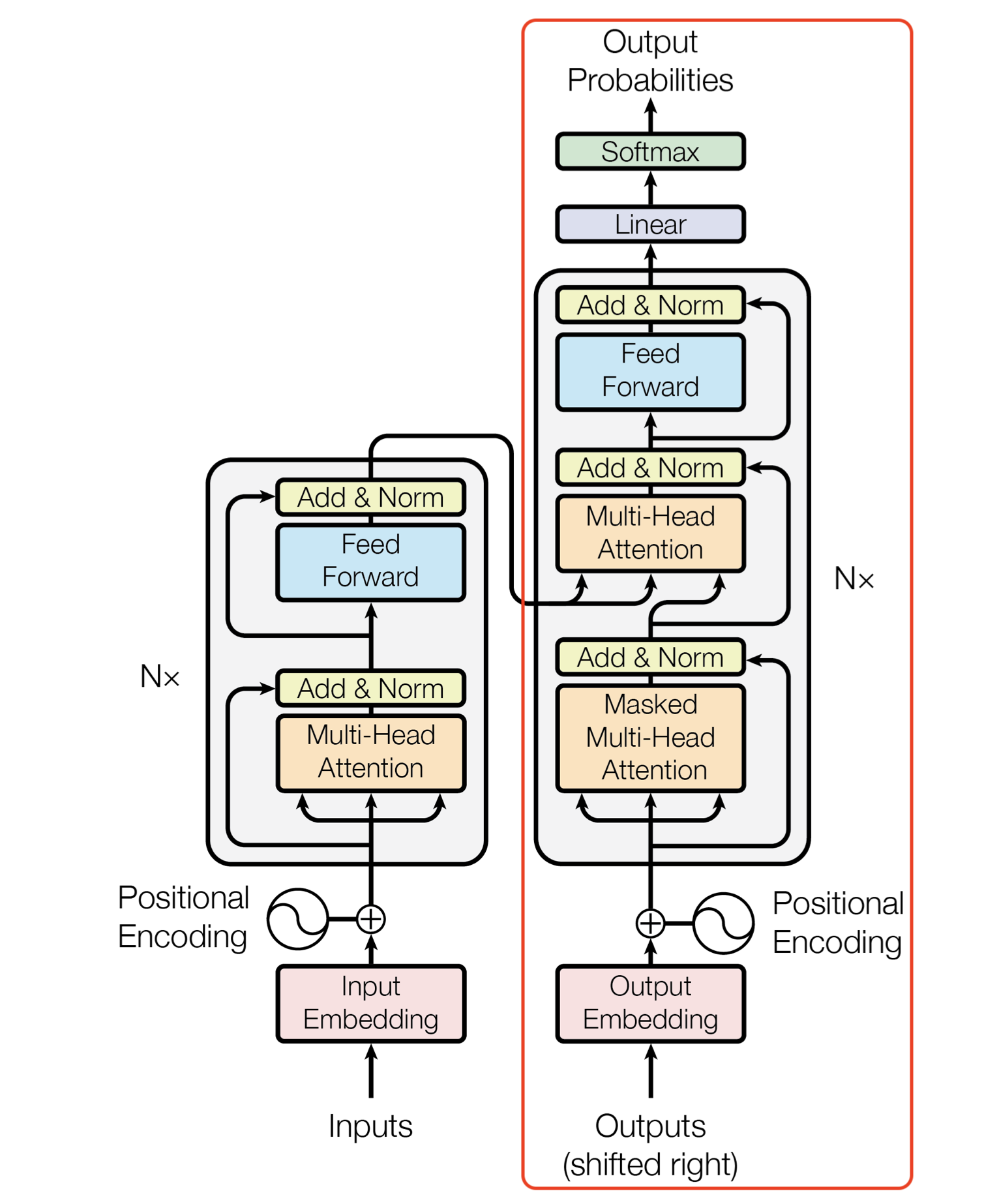 The Decoder Architecture
The Transformer decoder can be conceived as a conditional probability distribution that predicts the next possible token, considering both the encoded sentence in the source language and the previously predicted tokens. During training, when we supply the entire output sentence (the “answer”) but shift it one token to the right, we must apply a mask to prevent the decoder from simply peeking ahead and predicting the next token. The calculation of this mask can be observed in the implementation of the Transformer module.
class DecoderBlock(nn.Module):

    def __init__(self, in_features: int, hidden_features, n_attn_heads: int = 8):
        super().__init__()
        self._mh_attn_0 = MultiHeadAttention(in_features, n_attn_heads)
        self._mh_attn_1 = MultiHeadAttention(in_features, n_attn_heads)
        self._feed_forward = FeedForward(in_features, hidden_features, in_features)
        self._layer_norm_0 = LayerNorm(in_features)
        self._layer_norm_1 = LayerNorm(in_features)
        self._layer_norm_2 = LayerNorm(in_features)

        self._w_k_0 = nn.Linear(in_features, in_features)
        self._w_v_0 = nn.Linear(in_features, in_features)
        self._w_q_0 = nn.Linear(in_features, in_features)

        self._w_k_1 = nn.Linear(in_features, in_features)
        self._w_v_1 = nn.Linear(in_features, in_features)
        self._w_q_1 = nn.Linear(in_features, in_features)

    def forward(self, input: Dict):
        """Forward function of the decoder block. enc_out is expected from the encoder block."""

        x, enc_out = input['x'], input['enc_out']
        mask_tgt, mask_tgt_src = input['mask_tgt'], input['mask_tgt_src']

        x_0 = x
        x = self._layer_norm_0(x)
        q, k, v = self._w_q_0(x), self._w_k_0(x), self._w_v_0(x)
        x = self._mh_attn_0(q, k, v, mask=mask_tgt)  # mask_tgt is supposed to include the sequence length mask and the causal mask
        x += x_0
        del x_0

        x_1 = x
        x = self._layer_norm_1(x)
        v, k = self._w_v_1(enc_out), self._w_k_1(enc_out)
        q = self._w_q_1(x)
        x = self._mh_attn_1(q, k, v, mask=mask_tgt_src)  # mask_tgt_src is supposed to include the sequence length mask calculated from the src and tgt sequence jointly.
        x += x_1
        del x_1

        x_2 = x
        x = self._layer_norm_2(x)
        x = self._feed_forward(x)
        x += x_2
        del x_2

        return {'x': x, 'enc_out': enc_out, 'mask_tgt': mask_tgt, 'mask_tgt_src': mask_tgt_src}  # we keep the enc_out for the chained connection of decoder block
The Transformer
class Transformer(nn.Module):

    def __init__(
        self,
        dictionary_len: int,
        embedding_dim: int,
        embedding_padding_idx: int = 0,
        ff_hidden_features: int = 2048,
        n_encoder_blocks: int = 8,
        n_decoder_blocks: int = 8,
        n_attn_heads: int = 8,
    ):
        """Parameters:
        dictionary_len: the length of the dictionary, i.e. the number of tokens in the vocabulary
        embedding_dim: number of channels after the input & output embedding
        ff_hidden_features: the number of hidden features in the feed-forward layer
        n_encoder_blocks: number of encoder blocks
        n_decoder_blocks: number of decoder blocks
        n_attn_heads: number of attention heads
        """
        super().__init__()

        self._embedding_padding_idx = embedding_padding_idx
        self._embedding_dim = embedding_dim
        self._word_embedding = nn.Embedding(dictionary_len, embedding_dim, embedding_padding_idx)  # padding_idx depends on which index we use in the encoder for padding.
        self._encoder_blocks = nn.Sequential(*[EncoderBlock(embedding_dim, ff_hidden_features, n_attn_heads) for _ in range(n_encoder_blocks)])
        self._layer_norm_0 = LayerNorm(embedding_dim)
        self._decoder_blocks = nn.Sequential(*[DecoderBlock(embedding_dim, ff_hidden_features, n_attn_heads) for _ in range(n_decoder_blocks)])
        self._layer_norm_1 = LayerNorm(embedding_dim)
        self._pos_encoding = PositionalEncoding()

    def _get_masks(self, mask_type: str, src_tokens: Optional[Tensor] = None, tgt_tokens: Optional[Tensor] = None):
        """Calculate the mask to be feeded into the self attention calculation.
        'mask_type': type of mask
        'src_tokens': tensor of shape (B, seq_token),
        'tgt_tokens": tensor of shape (B, tgt_token),
        Returns:
            mask: shape (B, seq_len, seq_len) that can be applied to the attention module.
        """
        ignore_token_ids = [self._embedding_padding_idx]
        if mask_type == "src_mask":
            assert src_tokens is not None and tgt_tokens is None
            mask = get_mask_from_token(src_tokens, ignore_token_ids)
            mask_v = mask[:, None, :]  # B, 1, seq_len
            mask_h = mask[:, :, None]  # B, seq_len, 1
            mask = mask_v * mask_h  # B, seq_len, seq_len
        elif mask_type == "tgt_src_mask":
            assert tgt_tokens is not None and src_tokens is not None
            mask_tgt = get_mask_from_token(tgt_tokens, ignore_token_ids)[:, :, None]  # B, len_tgt, 1
            mask_src = get_mask_from_token(src_tokens, ignore_token_ids)[:, None, :]  # B, 1, len_src
            mask = mask_tgt * mask_src
        elif mask_type == "tgt_mask":
            assert tgt_tokens is not None and src_tokens is None
            mask = get_mask_from_token(tgt_tokens, ignore_token_ids)
            mask_v = mask[:, None, :]  # B, 1, seq_len
            mask_h = mask[:, :, None]  # B, seq_len, 1
            mask = mask_v * mask_h  # B, seq_len, seq_len
            mask &= torch.tril(mask)
        else:
            raise ValueError(f"Invalid mask_type={mask_type} given!")

        return mask


    def forward(self, input: Dict):
        """input is a dictionary containing the following keys:
        'source': batched input containing tokenized source language sentences stored as padded list of integers, shape (B, seq_len)
        'target': (Optional) batched input containing tokenized target language sentences stored as padded list of integers, shape (B, seq_len)
            in the inference time, target should be None, since the model will use it's own output at time t to condition its prediction at time t+1
        Note both source and target tensor have the same shape, because they share a joint vocabulary and also the embedding layer.

        The output is a tensor of shape (B, seq_len, dictionary_len) containing the probability distribution of the next token at each time step.
        """

        if self.training:
            src, tgt = input['source'], input['target']
            del input

            # in training time, we shift the target tensor by one time step to the right
            # and pad the first token with 0, which is the start of sequence token
            tgt = torch.cat([torch.zeros_like(tgt[:, 0:1]), tgt[:, :-1]], dim=-1)

            mask_src = self._get_masks("src_mask", src_tokens=src)
            mask_tgt = self._get_masks("tgt_mask", tgt_tokens=tgt)
            mask_tgt_src = self._get_masks("tgt_src_mask", src_tokens=src, tgt_tokens=tgt)

            rescale_factor = math.sqrt(self._embedding_dim)  # make it larger: we don't want the pe later to be louder than the words
            src = self._word_embedding(src) * rescale_factor
            tgt = self._word_embedding(tgt) * rescale_factor

            src = self._pos_encoding(src)
            tgt = self._pos_encoding(tgt)

            src_enc = self._layer_norm_0(self._encoder_blocks({'x': src, 'mask': mask_src})['x'])
            del src
            tgt_dec = self._layer_norm_1(self._decoder_blocks({'x': tgt, 'enc_out': src_enc, 'mask_tgt': mask_tgt, 'mask_tgt_src': mask_tgt_src})['x'])
            del src_enc

            tgt_dec = tgt_dec @ self._word_embedding.weight.T
            # tgt_dec = torch.softmax(tgt_dec, dim=-1)

            return tgt_dec

        else:
            src = input['source']
            tgt = torch.zeros_like(src)
            del input

            src_tokens = src
            mask_src = self._get_masks("src_mask", src_tokens=src)

            src = self._word_embedding(src)
            src = self._pos_encoding(src)
            src_enc = self._layer_norm_0(self._encoder_blocks({'x': src, 'mask': mask_src})['x'])
            del src

            tgt[:, 0] = self._embedding_padding_idx
            for i in range(tgt.shape[1]):
                mask_tgt = self._get_masks("tgt_mask", tgt_tokens=tgt)
                mask_tgt_src = self._get_masks("tgt_src_mask", src_tokens=src_tokens, tgt_tokens=tgt)
                tgt_dec = self._word_embedding(tgt)
                tgt_dec = self._pos_encoding(tgt_dec)
                tgt_dec = self._layer_norm_1(self._decoder_blocks({'x': tgt_dec, 'enc_out': src_enc, 'mask_tgt': mask_tgt, 'mask_tgt_src': mask_tgt_src})['x'])
                tgt_dec = tgt_dec @ self._word_embedding.weight.T
                # tgt_dec = torch.softmax(tgt_dec, dim=-1)
                next_tokens = tgt_dec[:, i, :].argmax(dim=-1)  # shape: (B,)
                if i != tgt.shape[1] - 1:
                    tgt[:, i+1] = next_tokens

            return tgt_dec
Byte-pair Encoding
Up to this point, I haven’t discussed how we convert sentences written in words into the numerical format that the transformer module can process, and vice versa. To bridge this gap, the authors utilized an algorithm known as Byte-pair Encoding (BPE). BPE iteratively identifies the most frequent byte pairs within a text corpus and constructs a lookup table mapping between strings and numerical representations.
Let’s illustrate this process with a simple example. Consider the sentence: "abababcd". Initially, assume we have a dictionary containing four alphabets: ['a', 'b', 'c', 'd'], each assigned an index [0, 1, 2, 3]. If we tokenize our sentence using this initial dictionary, we end up with an array [0, 1, 0, 1, 0, 1, 2, 3], which has a length of 8.
Byte-pair encoding effectively reduces the token length by expanding the initial dictionary with the most common token pairs. It starts by tallying the occurrences of each token pair. For our sentence, we count:
"a, b": 3
"b, a": 2
"b, c": 1
"c, d": 1
Since "a, b" is the most frequent token pair in the first iteration, we add it to our dictionary and re-tokenize our sentence. The new dictionary now becomes ['a', 'b', 'c', 'd', 'ab'], with indices [0, 1, 2, 3, 4]. Consequently, the tokenized array becomes [4, 4, 4, 2, 3].
This process continues until a stopping condition is met, typically when the dictionary reaches a certain size. The original authors created a dictionary containing 37,000 alphabets from a dataset of 4.5 million sentence pairs. However, due to hardware limitations, I opted for a smaller dataset (Multi30k) and consequently reduced my dictionary size to 1,000 alphabets.
You can find my implementation of the algorithm at the following locations: Link 1: BPE Algorithm, Link 2: BPE Learn Dictionary. The implementation has used a prefix tree (aka. Trie) data structure to reduce the tokenization time complexity from \(O(N^2)\) to \(O(N)\) with \(N\) being the sequence length. You can find my implementation of the trie in this link.
Lastly, it’s worth mentioning that if you’re working with language pairs that share many common alphabets, such as English and German, you might consider building a shared BPE for both languages. This allows you to share the same language embedding between the encoder and the decoder in the network, reducing the number of parameters needed and potentially mitigating overfitting.
Training Loop
The code for training this model can be accessed at the following location: Link.
Compared to the parameters used by the authors, I’ve reduced the model complexity to fit the training on my laptop-grade GPU which has only 6 GB of memory. In summary, here are the configurations of my lightweight model:
model_embedding_dim: int = 64
model_embedding_padding_idx: int = 2
model_ff_hidden_features: int = 256
model_encoder_blocks: int = 4
model_decoder_blocks: int = 4
model_attn_heads: int = 8
Below, I’ve included a few samples extracted from the log to illustrate how the model learns to translate German text into English. Special symbols like 𝄆 mark the beginning of a sentence, 𝄇 indicates the end of a sentence, and ♫ represents padded tokens. One can observe in the beginning the model struggles to predict meaningful results, and as the training progresses, it is able to pick up some common words, the start and stop signal of the sentence, but is still having difficulties for translating the whole sentence without any errors.
| Training Progress | Sample Predictions |
|---|---|
| Epoch 0 | |
| Input | 𝄆Männer in Anzug und Krawatte laufen die Treppe herunter.𝄇 |
| Prediction | ♫d, Men in Sons and SonAuwalking d, Sonmachngen eps𝄇 |
| Groundtruth | 𝄆Men in suits and ties walking downsteps𝄇 |
| Epoch 1 | |
| Input | 𝄆Ein Kind, das eine Papierkrone trägt und in einem Einkaufswagen sitzt.𝄇 |
| Prediction | ame 𝄆d, on GitarTa𝄇per crow𝄇sitting in a shwater.AuEin kleiner Junge 𝄇 |
| Groundtruth | 𝄆Kid wearing a paper crown sitting in a shopping cart.𝄇 |
| Epoch 16 | |
| Input | 𝄆Eine asiatische Frau steht neben Körben voller orangefarbener Früchte.𝄇 |
| Prediction | 𝄆An his e are a woman an woman stands on a sket on l of an vliit.𝄇 |
| Groundtruth | 𝄆There is an Asian woman standing near baskets full of orange fruits.𝄇 |
| Epoch 64 | |
| Input | 𝄆Ein Mann mit Brille, der an einem Tisch mit einer Kaffeetasse und mehreren anderen Gegenständen sitzt.𝄇 |
| Prediction | 𝄆A man with glasses is at a table with a coffee cup and smiveral other boems and table𝄇 |
| Groundtruth | 𝄆A man with glasses sitting at a table with a coffee cup and several other items on the table.𝄇 |
| Epoch 128 | |
| Input | 𝄆Drei schwarze Hunde sind an einem Strand.𝄇 |
| Prediction | 𝄆Three black dogs are on a beach.𝄇 |
| Groundtruth | 𝄆Three black dogs are on a beach.𝄇 |
Summary
In this blog post, we’ve taken a journey into the intricate world of the Transformer model, a groundbreaking neural architecture that has revolutionized various natural language processing tasks. Throughout our exploration, we’ve delved into the core components of the Transformer, including self-attention mechanisms, feed-forward layers, positional encoding, and layer normalization. We’ve also touched upon the essential pre-processing step of Byte-pair Encoding (BPE) to convert text data into numerical format.
While fun to implement, I am amazed at the Transformer’s ability to capture long-range dependencies in sequences, coupled with its parallel processing capabilities, has led to its widespread adoption and remarkable performance in tasks like machine translation, text generation, and language understanding. Its architecture has paved the way for numerous subsequent developments and adaptations.
As we continue our journey in the realm of deep learning and natural language processing, the Transformer serves as a foundational building block for exploring more advanced models and pushing the boundaries of what is possible in understanding and generating human language.
Feel free to explore the provided resources and references to delve even deeper into this fascinating field, and may your endeavors be guided by the power of the Transformer.